Descriptive statistics
In this article, I will lead you through the wonderful world of statistics, mostly descriptive statistics, and explain to you how to use this in Excel.
There is a saying stating:
There are three different kinds of lies: A white lie, a big lie, and statistics. Now, statistics make it possible to bend the truth to your will, but in order to do that, you will have to have a big understanding of statistics. It all begins with descriptive statistics.
Let’s start with a simple example and determine some statistical quantities. We will also take a look at the standard statistical function in Excel.
Take a look at the following numbers: 3, 3, 4, 5, 6, 7, 8, 8, 8, 9.
To calculate the average, we need to add all the numbers and divide it by the count:
Sum: 61,
Count: 10,
Average: 61/10=6.1.
Excel has the next known functions: SUM, COUNT, AVERAGE.
To expand the knowledge about the average relative to a data set and the other way around, statisticians came up with the next quantities:
The Median
The median is the middle value of a data set (when all the numbers are sorted from low to high). If there’s no middle value (when a data set has an even amount of numbers), the median is the average of the two middle values.
In our example, the two middle values are 6 and 7, so the median is (6+7)/2=6,5.
The median and the average are close together, which suggests that the distribution isn’t that big.
Quartiles
There are three quartiles, which are used to separate a data set into 4 groups. Then you can determine if the groups are somewhat evenly spread.
The second quartile is nothing more than the median.
The first quartile is the median of the group placed left of the median.
The third quartile is the median of the group placed right of the median.
In our example, the first quartile is 4, and the third is 8.
Excel knows the function QUARTILE, but this doesn’t always give the wanted result (this also applies to the two successors: QUARTILE.INC and QUARTILE.EXC) because these functions use percentiles and those are actually not important here.
Mode
The mode of a data set is the value that appears the most. If there are several values eligible for the mode, the mode doesn’t exist.
In our example, the mode is 8 because the number 8 occurs three times. If out 4 would have been a 3, the mode wouldn’t have existed.
Excel knows the function MODE (old) and MODE.SNGL to determine the mode. However, with this function, Excel will always give a result that is formally incorrect. When in our example 4 is changed to 3, the function MODE.SNGL will give 3 as the mode.
Variance
Another way to find the distribution is the variance. This is a tool to see how the data set values differ mutually.
To determine this, we need to do some work first.
The first step is to determine the difference with the average for every single value.
In our example we will get (resp.) -3,1; -3,1; -2,1; -1,1; -0,1; 0,1; 1,9; 1,9; 1,9; 2,9.
Now what would seem logical is to add all these numbers and divide them by the count (say the average of the differences). But this is where the dog catches its own tail. If we add all the differences, we end up with 0. That makes sense!
To prevent this, we need to get rid of the negatives (-). We can achieve this by squaring the differences.
We get: 9,61; 9,61; 4,41; 1,21; 0,01; 0,81; 3,61; 3,61; 3,61; 8,41.
The sum of the differences squared is 44,9. Excel has the function DEVSQ for this.
The variance can be reached by dividing the sum by the count. The variance is 44,9/10=4,49. This 4,49 tells us that the data set contains values between 6,1-4,49 and 6,1+4,49 (6,1 was the average), and that seems to be correct.
Now statisticians aren’t just liars, they also have a sensitive side. The variance we just calculated is actually too precise. We need to ‘loosen up’. You don’t need the variance of a population, but the variance of a sample.
But here lies a problem. Because this raises the question: What sample and what are the requirements for a sample? There’s no answer to this question.
To keep everything simple, they basically just said that the sample is one less!?!?
So to determine the variance of a sample, we need to divide the squared value by the count -1.
Okay, so the variance of the sample is 44,9/9=4,989. Fantastic!
The Excel functions for determining variances are VAR.P and VAR.S.
Standard deviation
The most important descriptive statistics is the standard deviation (SD).
This tells you something about the individual values relative to the average.
Suppose our numbers are the grades of 10 students taking a test. Are the ones with a 3 exceptionally bad and the ones with a 9 exceptionally good or not?
This question can be answered using the standard deviation.
But we have to calculate this first.
This is pretty easy if the variance is already calculated. The standard deviation is the square root of the variance. In our example, that is the square root of 4,49 = 2,12.
Keep in mind that the variance consists of squared numbers. To undo this, we need to take the square root to get to a standard. And that’s exactly what we do when calculating the standard deviation.
What does the standard deviation tell us?
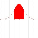
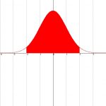
If the values are ‘normally’ divided, about 68% of the values are ranged from average-standard deviation to average+standard deviation and a good 98% ranged from average-2*standard deviation to average+2*standard deviation.
Our 68%-interval is [6,1-2,12..6,1+2,12] = [3,98..8,22] and our 95%-interval is [6,1-2*2,12..6,1+2*2,12] = [1,86..10,34].
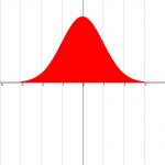
You could say that the 3’s and the 9’s fit perfectly into the 95%-interval and therefore aren’t exceptional. Everything outside the 95%-interval are considered ‘special’. Some statisticians work with a 99%-interval. This is the average +/-3*standard deviation. By the way, our population consisting of 10 is a little small to (normally) test, but that’s a side note.
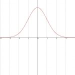
A normal distribution is usually examined using the intervals and of the values are evenly spread in those intervals. When you put this in a graph, you will get a clock-shape with a normal distribution.
Finally, I would like to point out that there is, of course, a standard deviation of a sample, which is the square root of the variance of the sample.
The Excel functions are STDEV.P and STDEV.S.
Minimum and Maximum
These two statistics are of course known.
The minimum is the smallest value and the maximum is the largest value.
In our example, the minimum is 3 and the maximum is 9.
In Excel, these functions are (resp.) MIN and MAX.
Classes
There are of course still statisticians who feel like it’s useful to subdivide values into classes and then calculate the average of each class or determine other statistics of each class. To me, it’s a mystery why one would still use classes in the time of computers and big-data-analysis. In the pre-computer time it was indeed useful to get rid of large amounts of data that way, but in times like these???
But, for these people, a rule of thumb:
A number of classes is the square root of a number of values and the class size is the absolute difference between the maximum and minimum divided by a number of classes.
Excel doesn’t have any functions or services for this.
Data statistics
The Excel-add-in Adequate from HJGSoft knows a couple of services to determine the standard statistics from a value series.
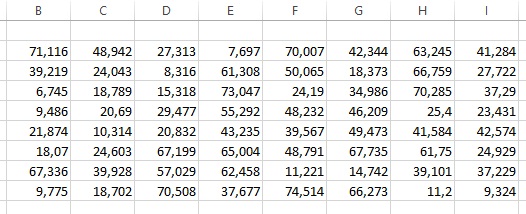
This example contains 64 measurements, completely randomly sorted. Before the statistics can be determined, the significance has to be determined first. After a brief consideration, that is 1 decimal: we would like to round every value to one decimal and use those numbers for the statistics.
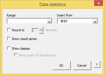
Click in the HJGSoft tab in the ribbon on the button Data Statistics.
The following window will pop up:
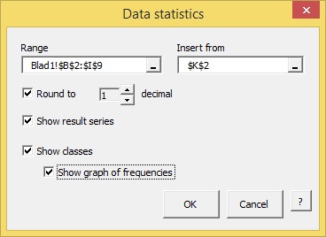
The options speak for themselves (in my opinion) and can be filled in like this:
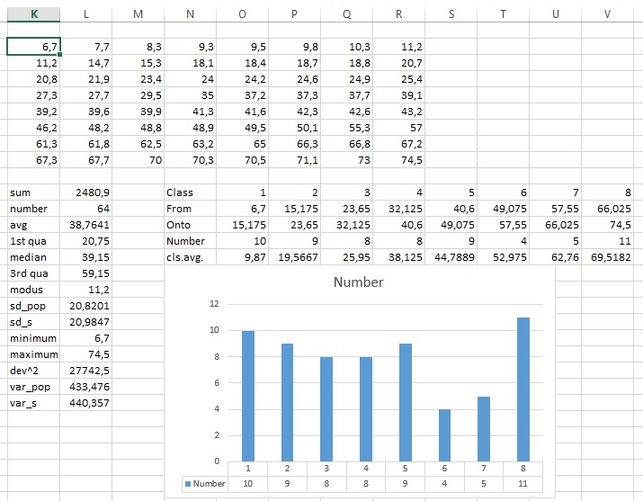
Press the OK button for the result:
MLRA is part of the Excel-Adequate of HJGSoft. For more information go to the page Excel Adequate. You can here download the tool and can try it out for free for 10 days.